The Kelly criterion calculates position size by maximizing expected compounded growth. It connects the probability of success, the payoff and the amount of capital exposed to loss. Its most useful lesson is also its least comfortable: a profitable strategy can still lose money through excessive sizing.
The calculation is straightforward. Estimating its inputs is not. A position that looks sensible with a 60% win probability can become excessive if the true probability is 55%. Kelly therefore needs to be treated as a model of capital allocation, not permission to trade whatever percentage a calculator produces.
What the Kelly Criterion Maximizes
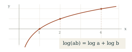
Kelly maximizes expected logarithmic wealth. Logarithms turn the multiplication involved in compounding into addition, allowing repeated gains and losses to be evaluated through a growth rate. This is the central idea developed in J. L. Kelly’s 1956 paper on information and capital growth.
Consider a position that increases an account by 20%, followed by another that reduces it by 20%. The account does not return to its starting value:
1.20 × 0.80 = 0.96
The result is a 4% loss. Equal percentage gains and losses do not cancel because each applies to a different capital balance.
Kelly accounts for this multiplication. It does not maximize the expected dollar profit from the next trade, minimize losses or guarantee the best result over a chosen trading period. Those are different objectives, and they can produce different position sizes.
The Kelly Formula for a Two-Outcome Bet
For a bet that either wins a fixed amount or loses the entire stake, define p as the probability of winning, q = 1 − p as the probability of losing, and b as the net profit per dollar staked on a win. The growth-maximizing fraction of current capital is:
f* = (bp − q) / b = p − q / b
This is a special case of the more general payoff formula in Edward Thorp’s analysis of Kelly sizing and optimal growth. The distinction between net profit and total payout matters: if a winning $1 stake returns $2 including the stake, then b equals 1, not 2.
A Worked Example
Suppose a hypothetical bet has a 55% probability of winning and pays $1 profit for every $1 staked. A loss forfeits that dollar:
f* = 0.55 − 0.45 / 1 = 0.10
Full Kelly therefore stakes 10% of current capital under these assumptions. With $10,000, the first stake is $1,000. After a loss, capital falls to $9,000 and the next stake becomes $900, assuming the probabilities and payoff remain unchanged.
The percentage stays constant; the dollar amount changes with the account. This example illustrates the mathematics, not a recommendation to risk 10% per trade.
If the formula produces zero or a negative number, the optimal allocation is zero when the available choices are taking that bet or holding cash. A negative result is not, by itself, an instruction to short an asset.
Risk Fraction Is Not Necessarily Position Value
In this example, f is the fraction lost on an unsuccessful bet. It is not automatically the fraction invested in shares, posted as collateral or committed as margin.
If a $10,000 account allocates $1,000 of planned loss exposure and each share has a planned $2 loss, the corresponding position is 500 shares before costs. If the actual loss becomes $3 per share, the account loses $1,500 instead. The original sizing calculation no longer describes the outcome.
Keep the capital fraction, dollar risk and position quantity separate. The conversion between them follows the same arithmetic used in fixed-fractional position sizing; Kelly supplies a proposed fraction rather than removing the need to measure exposure.
Why Positive Expected Value Is Not Enough
For the two-outcome model, expected profit per dollar staked is:
Expected profit = pb − q
With a 55% win probability and an even payoff, this equals $0.10. Increasing the stake increases expected dollar profit, but it also changes how losses affect future capital.
The expected logarithmic growth per opportunity is:
g(f) = p ln(1 + bf) + q ln(1 − f)
Substituting the example’s inputs gives g(0.10) of approximately 0.00501. At a 20% stake, g(0.20) is approximately −0.00014. Both stakes have positive expected dollar profit, yet the larger stake has negative expected log growth.
That is the distinction between a strategy’s expected value and its ability to compound capital at a chosen size. An edge identifies a potentially profitable opportunity. It does not make every allocation to that opportunity sensible.
The Assumptions Behind the Basic Calculation
The textbook example uses repeated independent outcomes with unchanged probabilities and payoffs. It allows capital to be divided as required and assumes positions can be resized after each result. The winning profit and losing amount are known in advance.
These assumptions describe the example, not every possible Kelly model. More advanced formulations can accommodate several assets, variable outcomes and conditional probabilities. They still require a defensible description of what can happen and how likely those outcomes are.
The growth rate also belongs to the model’s measurement period. Growth per completed trade is not annual growth. Converting between them requires assumptions about trade frequency, overlapping positions and how capital becomes available for reuse.
Finally, the capital base needs a clear definition. A trading account funded with money needed for near-term expenses has constraints that do not appear in the basic equation. Maximizing growth of that account does not establish that the resulting risk is affordable.
Estimation Risk: Small Input Errors, Large Sizing Changes
For an even payoff, b = 1, so the formula simplifies to:
f* = 2p − 1
Every percentage point added to the estimated win probability adds two percentage points to the calculated stake. The following figures are hypothetical model outputs:
| Assumed win probability | Calculated full Kelly fraction |
|---|---|
| 50% | 0% |
| 52% | 4% |
| 55% | 10% |
| 60% | 20% |
A trader estimating 60% would calculate a 20% stake. If the true probability were 55%, that allocation would be twice the true Kelly fraction. As the earlier calculation shows, it would also produce slightly negative expected log growth in this particular model.
Reducing positions can improve results when estimated inputs contain error. Simulations and tennis betting data in Baker and McHale’s research on betting under parameter uncertainty found improvements from shrinking estimated Kelly stakes. That finding does not establish one universally correct reduction for trading strategies.
A Historical Win Rate Is an Estimate
Suppose a strategy wins 55 of 100 trades. Its observed win rate is 55%, but the sample does not establish that its future win probability is exactly 55%.
Under an independent binary model with a constant win probability, the estimated standard error is:
√[0.55 × 0.45 / 100] ≈ 0.0497
That is approximately five percentage points. This calculation measures sampling uncertainty within the assumed model. It does not measure whether the model remains appropriate.
There is no universal trade count that makes Kelly reliable. The relevant question is whether uncertainty in the estimated edge remains large enough to change the sizing decision. More decimal places will not settle that question.
Payoffs Need the Same Scrutiny
Win probability is only half the estimation problem. Fees, execution costs and financing charges must be reflected in the outcomes being modeled. A historical payoff ratio that excludes those expenses describes a different opportunity from the one actually traded.
Test combinations of less favorable inputs rather than changing one number in isolation. A lower win rate accompanied by smaller winners or larger losses can alter the allocation far more than either change alone.
Kelly for Variable Returns and Multiple Positions
The familiar win-rate formula is exact for its stated two-outcome model. It is not a universal shortcut for a strategy with varying profits, varying losses and occasional extreme outcomes.
For a single opportunity with random return X per unit allocated, the broader objective is to choose f to maximize:
E[ln(1 + fX)]
The allocation must keep wealth positive across the modeled outcomes. With several simultaneous positions, the calculation evaluates their combined return, including dependence between them. These extensions appear in Thorp’s treatment of Kelly allocation in securities markets.
Because the logarithm is nonlinear, replacing every winner and loser with its respective average payoff does not generally preserve the correct answer. The distribution matters, not just its summary averages.
Dependence matters too. Suppose two positions each lose 10% of account capital when the same event occurs. Together they lose 20% in that event. Calculating each position independently does not make the combined exposure equivalent to two separate opportunities.
Why Use Fractional Kelly?
Fractional Kelly scales down the calculated allocation. Half Kelly uses 50% of the full Kelly amount; quarter Kelly uses 25%. If estimated full Kelly is 10%, these approaches allocate 5% and 2.5% respectively.
The practical purpose is to accept less modeled growth in exchange for lower exposure and more room for estimation errors. The choice still needs justification: half Kelly is a sizing rule, not proof that the remaining risk is acceptable.
The detailed comparison belongs in full Kelly versus fractional Kelly. For the basic calculation, the distinction is enough: the growth-maximizing output and the allocation actually used need not be identical.
Growth Optimal Does Not Mean Drawdown Safe
Return to the hypothetical 10% stake. Five consecutive losses reduce $10,000 to:
$10,000 × 0.905 = $5,904.90
That is a 40.95% decline. The position shrinks after each loss, but the account can still suffer a severe reduction.
Growth and acceptable downside can be modeled as separate requirements. Busseti, Ryu and Boyd’s research on risk-constrained Kelly allocation adds a constraint on the probability of wealth falling below a chosen fraction of starting capital. That is not the same as guaranteeing a maximum decline from every subsequent account peak.
Any modeled protection also depends on the assumed return distribution. An outcome excluded from the model is not controlled simply because the optimization produced a precise answer.
Using Kelly as Part of a Sizing Process
A practical application should make the assumptions visible before treating the result as usable:
- Define capital and outcomes. State what f measures and which losses the model permits.
- Estimate net returns. Include trading costs and avoid treating historical averages as known future values.
- Check sensitivity. Recalculate with weaker probabilities, worse payoffs and combined position exposure.
- Apply separate constraints. Set exposure, liquidity and loss limits that reflect the account’s purpose.
Kelly belongs within a broader position sizing and capital allocation process. It provides a disciplined connection between edge and exposure, while making the cost of overbetting explicit.
The strongest reason to calculate Kelly is not to obtain a large position size. It is to see how much that position depends on estimates being right. If modest changes in plausible inputs destroy the case for an allocation, the original number deserves less confidence, not more capital.